h[t] = H(h[t-1]).
We use a Softmax because we found that better results were obtained by discretizing the audio signals (also see van den Oord et al. (2016)) and outputting a Multinoulli distribution rather than using a Gaussian or Gaussian mixture to represent the conditional density of the original real-valued signal.The reference implementation by the original authors of the paper, sampleRNN_ICLR2017, is less readable (to me) than the PRiSM-SampleRNN implementation, so I'll use the second for the code dissection.
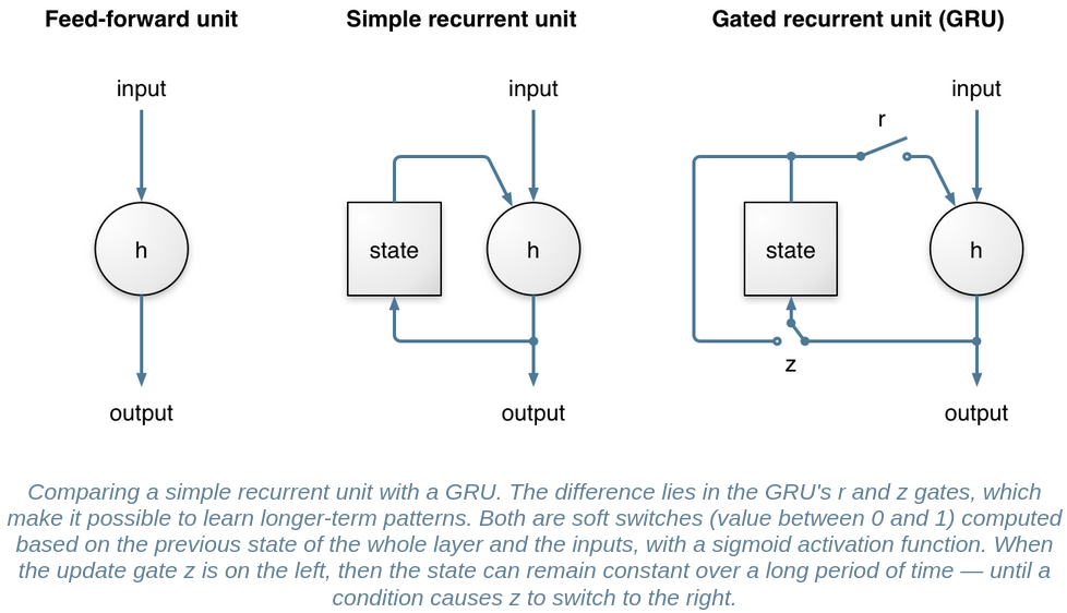
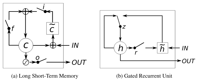
Recurrent neural networks (RNN) are very important here because they make it possible to model time sequences instead of just considering input and output frames independently. This is especially important for noise suppression because we need time to get a good estimate of the noise. For a long time, RNNs were heavily limited in their ability because they could not hold information for a long period of time and because the gradient descent process involved when back-propagating through time was very inefficient (the vanishing gradient problem). Both problems were solved by the invention of gated units, such as the Long Short-Term Memory (LSTM), the Gated Recurrent Unit (GRU), and their many variants.
RNNoise uses the Gated Recurrent Unit (GRU) because it performs slightly better than LSTM on this task and requires fewer resources (both CPU and memory for weights). Compared to simple recurrent units, GRUs have two extra gates. The reset gate controls whether the state (memory) is used in computing the new state, whereas the update gate controls how much the state will change based on the new input. This update gate (when off) makes it possible (and easy) for the GRU to remember information for a long period of time and is the reason GRUs (and LSTMs) perform much better than simple recurrent units.
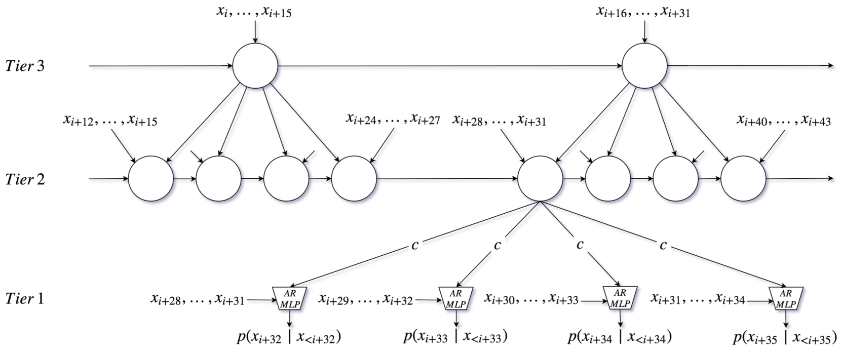
There's also a 3-tier option, but we initially had better results with 2-tier, so we don't use 3-tier. It doesn't have the modifications we made to 2-tier.
Table 1 and Figure 4 also show the 2-tier SampleRNN outperforming the 3-tier model in terms of likelihood and human rating respectively, which is very counterintuitive as one would expect longer-range temporal correlations to be even more relevant for music than for speech. This is not discussed at all, I think it would be useful to comment on why this could be happening.Author's reply:
"Why 2-tier is outperforming the 3-tier model for music?" - We did not expect that, but for any dataset and architecture structure, there is an optimal depth. Considering that this is a deep RNN (which introduces a form of recurrent depth, here very large) and the hypothesis that it is difficult to train such architectures in the first place, it is possible that alternative training procedures could yield better results with a deeper model.
    self.inputs = tf.keras.layers.Conv1D(
        filters=self.dim, kernel_size=frame_size, use_bias=False
    )
    self.hidden = tf.keras.layers.Dense(self.dim, activation='relu')
    self.outputs = tf.keras.layers.Dense(self.q_levels, activation='relu')
An MLP is a simpler, more primitive precursor to the more complex CNN (convolutional neural network like WaveNet) or RNN[4]. This choice is described in the paper as saving computation cost since the sample-to-sample relationship among nearby samples is probably a simple one. They're implying that the more complex non-linearities of music are in the higher tiers, and that small local clusters of samples have a simpler relationships.
    class SampleMLP(tf.keras.layers.Layer):

        def __init__(self, frame_size, dim, q_levels, emb_size):
            self.inputs = tf.keras.layers.Conv1D(
                filters=self.dim, kernel_size=frame_size, use_bias=False
            )
            self.hidden = tf.keras.layers.Dense(self.dim, activation='relu')
            self.outputs = tf.keras.layers.Dense(self.q_levels, activation='relu')

        def call(self, inputs, conditioning_frames):
            batch_size = tf.shape(inputs)[0]

            inputs = self.embedding(tf.reshape(inputs, [-1]))
            inputs = self.inputs(tf.reshape(inputs, [batch_size, -1, self.q_levels]))

            hidden = self.hidden(inputs + conditioning_frames)
            return self.outputs(hidden)
Note how the externally-passed conditioning is added to the model's own hidden layers. Another notable feature is that the inputs to the MLP have a 1D convolution applied. This is not described in the paper, but a hybrid Conv1D-MLP model does exist in literature[5]. It looks to me like in this implementation choice (PRiSM), they applied a hybrid Conv1D/MLP approach, especially since the reference SampleRNN implementation[6] does not have any 1D convolutions in the SampleRNN code.
As in the conventional 2D CNNs, the input layer is a passive layer that receives the raw 1D signal and the output layer is a MLP layer with the number of neurons equal to the number of classesThis seems to fit - the convention carried over from conventional 2D CNN models, since the SampleMLP has the same number of outputs as the quantization channels (256).
Unlike to the traditional recurrent unit which overwrites its content at each time-step (see Eq. (2)), an LSTM unit is able to decide whether to keep the existing memory via the introduced gates. Intuitively, if the LSTM unit detects an important feature from an input sequence at early stage, it easily carries this information (the existence of the feature) over a long distance, hence, capturing potential long-distance dependencies.The introduction to GRU describes the importance of GRUs to capturing dependencies on different time scales:
A gated recurrent unit (GRU) was proposed by Cho et al. [2014] to make each recurrent unit to adaptively capture dependencies of different time scaleThe actual gated units resemble some gated logic processors:
    class FrameRNN(tf.keras.layers.Layer):
        def __init__(self, rnn_type, frame_size, num_lower_tier_frames, num_layers, dim, q_levels, skip_conn):
            super(FrameRNN, self).__init__()
            self.skip_conn = skip_conn
            self.inputs = tf.keras.layers.Dense(self.dim)
            self.rnn = RNN(rnn_type, self.dim, self.num_layers, self.skip_conn)

        def build(self, input_shape):
            self.upsample = tf.Variable(
                tf.initializers.GlorotNormal()(
                    shape=[self.num_lower_tier_frames, self.dim, self.dim]),
                name="upsample",
            )

        def call(self, inputs, conditioning_frames=None):
            batch_size = tf.shape(inputs)[0]

            input_frames = tf.reshape(inputs, [
                batch_size,
                tf.shape(inputs)[1] // self.frame_size,
                self.frame_size
            ])
            input_frames = ( (input_frames / (self.q_levels / 2.0)) - 1.0 ) * 2.0
            num_steps = tf.shape(input_frames)[1]

            input_frames = self.inputs(input_frames)

            if conditioning_frames is not None:
                input_frames += conditioning_frames

            frame_outputs = self.rnn(input_frames)
Interesting to note is that skip connections are used in the code but not mentioned in the paper. As covered, skip connections in WaveNet were to solve the vanishing gradient problem - but, in SampleRNN, the use of GRUs (or LSTMs) in the RNN should hypothetically solve the vanishing gradient problem. However, there is support in literature for skip RNNs[9] - perhaps combining both brings even better performance.
    class SampleRNN(tf.keras.Model):
        def __init__(self, batch_size, frame_sizes, q_levels, q_type,
                     dim, rnn_type, num_rnn_layers, seq_len, emb_size, skip_conn):
            super(SampleRNN, self).__init__()
            self.big_frame_size = frame_sizes[1]
            self.frame_size = frame_sizes[0]

            self.big_frame_rnn = FrameRNN(
                frame_size = self.big_frame_size,
    	    )

            self.frame_rnn = FrameRNN(
                frame_size = self.frame_size,
    	    )

            self.sample_mlp = SampleMLP(
                self.frame_size, self.dim, self.q_levels, self.emb_size
            )
        # Inference
        @tf.function
        def inference_step(self, inputs, temperature):
            num_samps = self.big_frame_size
            samples = inputs
            big_frame_outputs = self.big_frame_rnn(tf.cast(inputs, tf.float32))
            for t in range(num_samps, num_samps * 2):
	        frame_inputs = samples[:, t - self.frame_size : t, :]
	        big_frame_output_idx = (t // self.frame_size) % (
                    self.big_frame_size // self.frame_size
                )
                frame_outputs = self.frame_rnn(
                    tf.cast(frame_inputs, tf.float32),
                    conditioning_frames=unsqueeze(big_frame_outputs[:, big_frame_output_idx, :], 1))
                sample_inputs = samples[:, t - self.frame_size : t, :]
                sample_outputs = self.sample_mlp(
                    sample_inputs,
                    conditioning_frames=unsqueeze(frame_outputs[:, frame_output_idx, :], 1))

        def call(self, inputs, training=True, temperature=1.0):
            if training==True:
                # UPPER TIER
                big_frame_outputs = self.big_frame_rnn(
                    tf.cast(inputs, tf.float32)[:, : -self.big_frame_size, :]
                )
                # MIDDLE TIER
                frame_outputs = self.frame_rnn(
                    tf.cast(inputs, tf.float32)[:, self.big_frame_size-self.frame_size : -self.frame_size, :],
                    conditioning_frames=big_frame_outputs,
                )
                # LOWER TIER (SAMPLES)
                sample_output = self.sample_mlp(
                    inputs[:, self.big_frame_size - self.frame_size : -1, :],
                    conditioning_frames=frame_outputs,
                )
                return sample_output
            else:
                return self.inference_step(inputs, temperature)
We can see the results of the 3 tiers cascading down into the lower tier, influencing the generation of the final waveform. The actual waveform results are created by the call functions of the Sample MLP and Frame RNNs shown above.
train.py:
    def create_adam_optimizer(learning_rate, momentum):
        return tf.optimizers.Adam(learning_rate=learning_rate,
                                  epsilon=1e-4)

    def create_sgd_optimizer(learning_rate, momentum):
        return tf.optimizers.SGD(learning_rate=learning_rate,
                                 momentum=momentum)

    def create_rmsprop_optimizer(learning_rate, momentum):
        return tf.optimizers.RMSprop(learning_rate=learning_rate,
                                     momentum=momentum,
                                     epsilon=1e-5)

    optimizer_factory = {'adam': create_adam_optimizer,
                     'sgd': create_sgd_optimizer,
                     'rmsprop': create_rmsprop_optimizer}

    # Optimizer
    opt = optimizer_factory[args.optimizer](
        learning_rate=args.learning_rate,
        momentum=args.momentum,
    )

    # Compile the model
    compute_loss = tf.keras.losses.SparseCategoricalCrossentropy(from_logits=True)
    train_accuracy = tf.keras.metrics.SparseCategoricalAccuracy(name='accuracy')
    model.compile(optimizer=opt, loss=compute_loss, metrics=[train_accuracy])
These are passed into the SampleRNN model code (samplernn/model.py):
    def train_step(self, data):
        (x, y) = data
        with tf.GradientTape() as tape:
            raw_output = self(x, training=True)
            prediction = tf.reshape(raw_output, [-1, self.q_levels])
            target = tf.reshape(y, [-1])
            loss = self.compiled_loss(
                target,
                prediction,
                regularization_losses=self.losses)
        grads = tape.gradient(loss, self.trainable_variables)
        grads, _ = tf.clip_by_global_norm(grads, 5.0)
        self.optimizer.apply_gradients(zip(grads, self.trainable_variables))
        self.compiled_metrics.update_state(target, prediction)
        return {metric.name: metric.result() for metric in self.metrics}
Like with WaveNet, a predicted waveform is produced from the model during training and then compared to the input waveforms to compute the loss. The actual prediction is done with self(x, training=True), which in Python would be implemented by the object's call() function:
    def call(self, inputs, training=True, temperature=1.0):
       # UPPER TIER
       big_frame_outputs = self.big_frame_rnn(
           tf.cast(inputs, tf.float32)[:, : -self.big_frame_size, :]
       )
       # MIDDLE TIER
       frame_outputs = self.frame_rnn(
           tf.cast(inputs, tf.float32)[:, self.big_frame_size-self.frame_size : -self.frame_size, :],
           conditioning_frames=big_frame_outputs,
       )
       # LOWER TIER (SAMPLES)
       sample_output = self.sample_mlp(
           inputs[:, self.big_frame_size - self.frame_size : -1, :],
           conditioning_frames=frame_outputs,
       )
       return sample_output
The values are 16-sample frames for the middle tier, and 64-sample frames for the upper tier.
Here we see a key distinction between SampleRNN and WaveNet. WaveNet uses the weights of the dilated convolution network to predict samples with knowledge of different temporal scales built in. SampleRNN is using patterns learned at broad temporal scales to condition the lower temporal scales - this means that SampleRNN's choice of high-level/long-term temporal feature feeds into the subsequent choices for the low-level temporal feature predictions.
softmax_cross_entropy_with_logits function[10], while SampleRNN uses a slightly different API[11],SparseCateoricalCrossentropy. The difference is explained simply that if your data is one-hot encoded (i.e. 256-bit mu-law integers expanded into a vector of 256 0s or 1s, like WaveNet), you would use the softmax cross entropy function, whereas if they're integers (like SampleRNN), you would use a sparse softmax cross entropy function.
    initial_epoch = get_initial_epoch(resume_from)
    dataset = get_dataset(args.data_dir, args.num_epochs-initial_epoch, args.batch_size, seq_len, overlap)

    # Dataset iterator
    def train_iter():
        for batch in dataset:
            num_samps = len(batch[0])
            for i in range(overlap, num_samps, seq_len):
                x = quantize(batch[:, i-overlap : i+seq_len], q_type, q_levels)
                y = x[:, overlap : overlap+seq_len]
                yield (x, y)

    callbacks = [
        TrainingStepCallback(
            model = model,
            num_epochs = args.num_epochs,
            steps_per_epoch = steps_per_epoch,
            steps_per_batch = steps_per_batch,
        ModelCheckpointCallback(
            monitor = 'loss',
            save_weights_only = True,
            save_best_only = args.checkpoint_policy.lower()=='best',
            save_freq = args.checkpoint_every * steps_per_epoch),
        tf.keras.callbacks.EarlyStopping(
            monitor = 'loss',
            patience = args.early_stopping_patience),
    ]
The above code is the equivalent of the training loop of WaveNet, where the SampleRNN model exposes its trainable variables and the Tensorflow library is leveraged to use the loss function above to train the model.