Hybrid approaches

Deficiencies of purely neural approaches

The author of RNNoise^[1],[2], a hybrid machine-learning/DSP approach to noise suppression (adopted in the popular VoiP project Mumble), states:

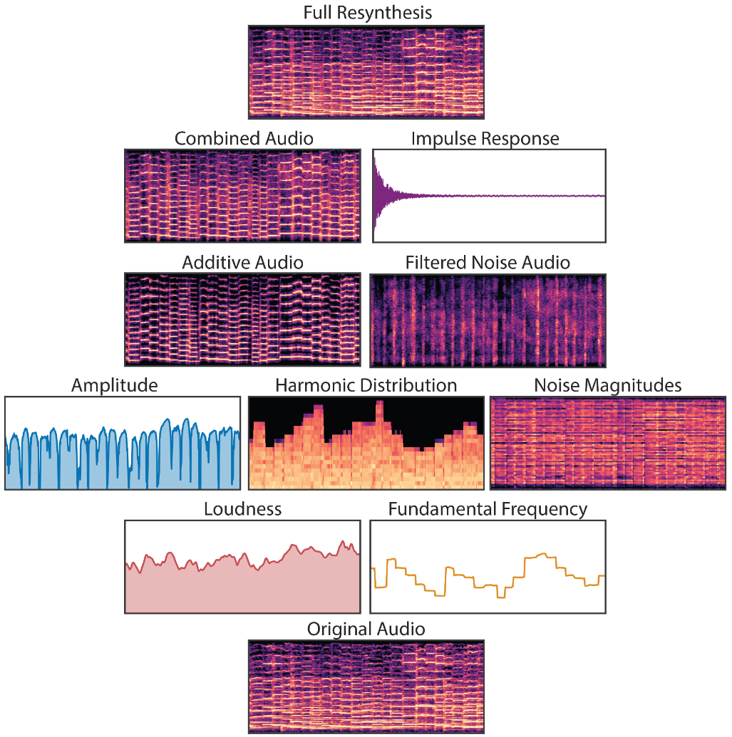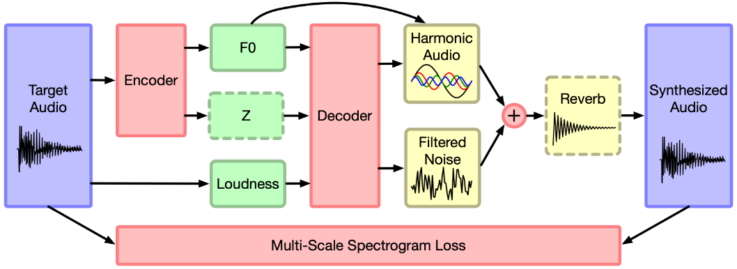
Thanks to the successes of deep learning, it is now popular to throw deep neural networks at an entire problem. These approaches are called end-to-end — it's neurons all the way down. End-to-end approaches have been applied to speech recognition and to speech synthesis On the one hand, these end-to-end systems have proven just how powerful deep neural networks can be. On the other hand, these systems can sometimes be both suboptimal, and wasteful in terms of resources. For example, some approaches to noise suppression use layers with thousands of neurons — and tens of millions of weights — to perform noise suppression. The drawback is not only the computational cost of running the network, but also the size of the model itself because your library is now a thousand lines of code along with tens of megabytes (if not more) worth of neuron weights.

This is different from the primary rationale presented by the authors of Magenta DDSP^[3],[4] in presenting their library:

Neural networks (such as WaveNet or GANSynth) are often black boxes. They can adapt to different datasets but often overfit details of the dataset and are difficult to interpret.

These arguments aren't mutually exclusive - an overly large or computationally complex model is probably also one that is a black box, or difficult to understand.

Magenta DDSP

Magenta is a collection of differentiable (i.e. can be trained and learn parameters with typical machine learning methods) DSP building blocks: oscillators, filters, etc.^[3]:

In the paper's introduction^[5] they make the case for why we should want to incorporate physical models and traditional DSP:

The bias of the natural world is to vibrate. Second-order partial differential equations do a surprisingly good job of approximating the dynamics of many materials and media, with physical perturbations leading to harmonic oscillations (Smith, 2010). Accordingly, human hearing has evolved to be highly sensitive to phase-coherent oscillation, decomposing audio into spectrotemporal responses through the resonant properties of the basilar membrane and tonotopic mappings into the auditory cortex (Moerel et al., 2012; Chi et al., 2005; Theunissen & Elie, 2014). However, neural synthesis models often do not exploit these same biases for generation and perception.

Paper overview

The paper^[5] starts off with some high-level criticisms of end-to-end neural approaches to audio, including WaveNet and SampleRNN:

The 3 criticisms are respectively:

strided convolution models–such as SING (Defossez et al., 2018), MCNN (Arik et al., 2019), and WaveGAN (Donahue et al., 2019)–generate waveforms directly with overlapping frames. Since audio oscillates at many frequencies, all with different periods from the fixed frame hop size, the model must precisely align waveforms between different frames and learn filters to cover all possible phase variations

Fourier-based models–such as Tacotron (Wang et al., 2017) and GANSynth (Engel et al., 2019)–also suffer from the phase-alignment problem, as the Short-time Fourier Transform (STFT) is a representation over windowed wave packets. Additionally, they must contend with spectral leakage, where sinusoids at multiple neighboring frequencies and phases must be combined to represent a single sinusoid when Fourier basis frequencies do not perfectly match the audio

Autoregressive waveform models–such as WaveNet (Oord et al., 2016), SampleRNN (Mehri et al.,2016), and WaveRNN (Kalchbrenner et al., 2018)–avoid these issues by generating the waveform a single sample at a time. They are not constrained by the bias over generating wave packets and can express arbitrary waveforms. However, they require larger and more data-hungry networks, as they do not take advantage of a bias over oscillation. Furthermore, the use of teacher-forcing during training leads to exposure bias during generation, where errors with feedback can compound. It also makes them incompatible with perceptual losses such as spectral features (Defossez et al.,2018), pretrained models (Dosovitskiy & Brox, 2016), and discriminators (Engel et al., 2019). This adds further inefficiency to these models, as a waveform’s shape does not perfectly correspond to perception

Case studies - learned violin synthesizer

The main examples used in the paper is a violin auto-encoder, trained on a mere 13 minutes of violin performance data:

Using the MusOpen royalty free music library, we collected 13 minutes of expressive, solo violin performances.

This is a huge reduction in the amount of training data required (e.g. 10 hours of piano performances were used to train WaveNet), by incorporating knowledge of the physical world and the human auditory system in the network.

Results:

Decomposition of a clip of solo violin. Audio is visualized with log magnitude spectrograms. Loudness and fundamental frequency signals are extracted from the original audio. The loudness curve does note exhibit clear note segmentations because of the effects of the room acoustics. The DDSP decoder takes those conditioning signals and predicts amplitudes, harmonic distributions, and noise magnitudes. Note that the amplitudes are clearly segmented along note boundaries without supervision and that the harmonic and noise distributions are complex and dynamic despite the simple conditioning signals. Finally, the extracted impulse response is applied to the combined audio from the synthesizers to give the full resynthesis audio.

RNNoise

In RNNoise^[1], first a typical noise reduction block diagram is considered:

Then, each block is replaced with a neural formulation:

The authors use Bark frequency bands to reduce the dimensionality of their inputs (as we've seen, high dimensionality is probably the most common problem of direct-from-waveform learning approaches).

The most interesting aspect of RNNoise (in my opinion) is that the end result for inference is a lightweight C library which performs real-time inference. The Python training scripts, after learning coefficients, generate the appropriate C source and header files in the final library.

Unfortunately, RNNoise's code^[2] is in bad shape - the README and instructions do not presently work, and one has to scour the GitHub issues to figure out the magic incantations. Despite being a hybrid ML/DSP approach, it suffers from the same deficiencies as many of the purely-neural codebases that I examined throughout this project (instructions don't work, unanswered reproducibility concerns, etc.).

Code dive

Despite my trouble in running or training RNNoise myself, I can still do a precursory code dive alongside an analysis of the paper^[6]. There is more detailed block diagram in the paper:

Alongside it is the description:

The signal-level block diagram for the system is shown in Fig. 2. The bulk of the suppression is performed on a low-resolution spectral envelope using gains computed from a recurrent neural network (RNN). Those gains are simply the square root of the ideal ratio mask (IRM). A finer suppression step attenuates the noise between pitch harmonics using a pitch comb filter.

Python neural training code

The training code^[2] is located in training/rnn_train.py:

    main_input = Input(shape=(None, 42), name='main_input')
    tmp = Dense(24, activation='tanh', name='input_dense', kernel_constraint=constraint, bias_constraint=constraint)(main_input)
    vad_gru = GRU(24, activation='tanh', recurrent_activation='sigmoid', return_sequences=True, name='vad_gru', kernel_regularizer=regularizers.l2(reg), recurrent_regularizer=regularizers.l2(reg), kernel_constraint=constraint, recurrent_constraint=constraint, bias_constraint=constraint)(tmp)
    vad_output = Dense(1, activation='sigmoid', name='vad_output', kernel_constraint=constraint, bias_constraint=constraint)(vad_gru)
    noise_input = keras.layers.concatenate([tmp, vad_gru, main_input])
    noise_gru = GRU(48, activation='relu', recurrent_activation='sigmoid', return_sequences=True, name='noise_gru', kernel_regularizer=regularizers.l2(reg), recurrent_regularizer=regularizers.l2(reg), kernel_constraint=constraint, recurrent_constraint=constraint, bias_constraint=constraint)(noise_input)
    denoise_input = keras.layers.concatenate([vad_gru, noise_gru, main_input])
    
    denoise_gru = GRU(96, activation='tanh', recurrent_activation='sigmoid', return_sequences=True, name='denoise_gru', kernel_regularizer=regularizers.l2(reg), recurrent_regularizer=regularizers.l2(reg), kernel_constraint=constraint, recurrent_constraint=constraint, bias_constraint=constraint)(denoise_input)
    
    denoise_output = Dense(22, activation='sigmoid', name='denoise_output', kernel_constraint=constraint, bias_constraint=constraint)(denoise_gru)
    
    model = Model(inputs=main_input, outputs=[denoise_output, vad_output])
    
    model.compile(loss=[mycost, my_crossentropy],
                  metrics=[msse],
                  optimizer='adam', loss_weights=[10, 0.5])

We can see most of the traits of the paper reproduced faithfully in the model code, which is very concise:

The input features are of size 42, which consists of BFCCs (Bark-frequency cepstral coefficients) and some others:
we apply a DCT on the log spectrum, which results in 22 Bark-frequency cepstral coefficients (BFCC). In addition to these, we also include the temporal derivative and the second temporal derivative of the first 6 BFCCs. We compute the DCT of the pitch correlation across frequency bands and include the first 6 coefficients in our set of features. At last, we include the pitch period as well as a spectral non-stationarity metric that can help in speech detection. In total we use 42 input features.
There are 3 distinct neural blocks that roughly correspond to the 3 traditional DSP components of a denoiser:
1. vad_gru: vad == Voice-Activity Detection
2. noise_gru: Noise Spectral Estimation
3. denoise_gru: Spectral Subtraction
However, note the author's warnings in the paper^[6]:
The design is based on the assumption that the three recurrent layers are each responsible for one of the basic components from Fig. 1. Of course, in practice the neural network is free to deviate from this assumption (and likely does to some extent).
and their demo website^[1]:
Of course, as is often the case with neural networks we have no actual proof that the network is using its layers as we intend, but the fact that the topology works better than others we tried makes it reasonable to think it is behaving as we designed it.

The training code is meant to be run with supplied signal and noise examples (in the raw/pcm format). Each of these is loaded into the appropriate neural blocks as the input, but this is done indirectly with some other tools. Recall that unlike WaveNet and SampleRNN, RNNoise is trained not on the waveform, but a new transform of 42 features (including 22 BFCCs and some pitch features).

The instructions are in TRAINING-README:

    (1) cd src ; ./compile.sh
    
    (2) ./denoise_training signal.raw noise.raw count > training.f32
    
        (note the matrix size and replace 500000 87 below)
    
    (3) cd training ; ./bin2hdf5.py ../src/training.f32 500000 87 training.h5
    
    (4) ./rnn_train.py
    
    (5) ./dump_rnn.py weights.hdf5 ../src/rnn_data.c ../src/rnn_data.h

There is a matrix created which is then ingested by the rnn_train.py script to load the features of signal and noise for training the neural layers.

It's unclear how to load more than one file, but other users on GitHub mentioned concatenating all of their signal and all of their noise clips into two giant raw files.

Generated C code with learned coefficients

The step after training is to use the script training/dump_rnn.py to dump the learned coefficients into C source and header files for the final RNNoise library, in src/rnn_data.c:

    static const rnn_weight input_dense_weights[1008] = {
       -15, 11, 11, 35, 37, 51, -56, -3,
       -53, -55, 20, -7, -94, 2, -54, 23,
       ...
    };
    
    static const rnn_weight input_dense_bias[24] = {
       5, 16, 9, 7, 0, -15, 11, -7,
       12, 7, 10, -10, 6, -15, 11, 7,
       -8, 11, -11, -21, -11, -19, -14, -14
    };
    
    static const DenseLayer input_dense = {
       input_dense_bias,
       input_dense_weights,
       42, 24, ACTIVATION_TANH
    };
    
    static const rnn_weight vad_gru_weights[1728] = {
       -35, -49, -33, -4, 40, -49, 24, -27,
       28, -61, 57, -30, -65, -82, 19, 61,
       -22, 42, 57, -61, 3, -18, -46, -31,
       ...
    };

There are thousands of lines and weights, but this in fact reminds me of when I optimized BTrack (a pure-DSP beat tracking algorithm) on an Android phone, and precomputed some magic coefficient arrays. The point to the comparison is that the idea of arrays full of hardcoded coefficients is not unusual in the DSP realm.

The actual C code which does inference (i.e. the step after training when the neural network actually does the function it was trained to do - i.e. in this case eliminate noise), by executing the feed-forward GRUs with the trained weights, is the core of RNNoise - but it's complex and I will skip the analysis.